Most articles introducing machine learning on the web start out with charts and equations showing how to fit a line to a linearly separable point cloud. That’s neat. But that does nothing to show the power of machine learning models to change the way that we write software and conduct business. There will be plenty of technical terms in this article, but I promise there will be absolutely no charts or equations. Let’s get down to business…

It’s Really Not that Fancy

The machine part is pretty obvious, usually we are talking about digital computers–servers in the cloud, our smartphones, tablets, etc. What exactly do we mean when we say a digital computer learns?

Supervised Learning is a process by which a digital computer learns to make useful inferences from the environment by being explicitly taught. For example, predicting the future price of a stock based on key factors affecting the business and it’s historical stock prices.

Unsupervised Learning is a process by which a digital computer learns to make useful inferences without being explicitly taught. Since the outputs haven’t been explicitly described, this process is more useful for identifying important relationships rather than making decisions. For example, making a map of social influencers on Twitter.

Reinforcement Learning is a process by which a digital computer can automatically improve the accuracy of its inferences. For example, getting better at controlling a vehicle by running over fewer and fewer cats. The initial model the computer uses is often created via training.

All three processes follow the same general algorithm:

1. Sense: Gather input from the environment. This could involve looking at pixel data from a CCD camera to see, read values from an accelerometer to detect motion, or even download a financial report or stock quote if we are trying to sense the financial world instead of the physical world.
2. Predict: Make inferences by applying the sensory data to an internal model. Is the cat going to land on its feet? Is the stock market about to crash? Is that Sally? How old is she?
3. Evaluate: Determine whether the inferences were correct. “Oops. That wasn’t Sally!” or “I should have left that cash under the mattress.”
4. Refine: Update the internal model given the feedback provided in Step 3.

Where the different learning approaches differ is in how they handle Step 3: Evaluate.

In Supervised Learning, the computer can check with an external agent, such as a person or the historical record to perform the evaluation. The hope is that eventually the training wheels can be removed and the computer will continue to make “good enough” inferences.

In Unsupervised Learning, we don’t care whether the computer is correct to some external measure. So the computer makes up its own evaluation metric based on the size and shape of the sensory data.

In Reinforcement Learning, the environment reacts to the inference made by the computer, which helps it evaluate the correctness of the inference.

It turns out that there isn’t just one way humans can set up models for the computer to learn with because we ourselves have not been able to devise a universal model that that explains the meaning of life, the universe, and everything. Instead, we solve this problem by devising algorithms that work well with different kinds of sensory input.

Models

Machine learning models are statistical models. A statistical model is an algorithm that works on a set of data and makes inferences. Each algorithm is usually supported by a set of mathematical specifications and proofs. But we’ll leave that for another day.

Types of Models

Models are grouped based on three classifications of problems:

1. Binary Classification: These can answer questions like “Am I wearing pants?” where there is a yes/no answer.
2. Multi-class or Multi-label Classification: These can answer questions like “What kind of pants am I wearing?” where there is more than one category of answer.
3. Regression: These can answer questions like “How much are my pants worth, how big are they, and where can I change them?” where the answer is a continuous number.

Anatomy of a Model

There are four components of a machine learning model:

1. The Training Algorithm: This is the process by which the model can learn from the data.
2. The Training Parameters: These are the parameters that customize the training algorithm for the type of problem you are trying to solve. The training algorithm paired with the training parameters is often called an Untrained Model.
3. The Inference Algorithm: There are several kinds of inferences you can make from data and they each have their own sub-field of machine learning dedicated to them.
4. The Inference Parameters: These are the parameters of the model learned from the training data as opposed to set beforehand. The pair of the Inference Algorithm and Inference Parameters is often referred to as a Trained Model.

Inference Algorithms

Most of the media hype surrounding machine learning concentrates on novel inference algorithms. Technologies like IBM Watson rely on breakthroughs in this area. Here are some of the most widely used algorithms:

Decision Trees

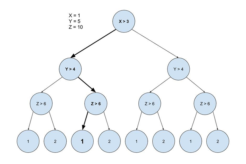
Decision Trees are an easily grasped algorithm. The inspiration of the algorithm is how we perceive our own inference process. If x is true, then y. If y is true, then z. If you’ve ever made a flow chart of a process in a business, or made a pros and cons table, then you’ve made a decision tree (Ha, see what I did there?). Decision trees chain a series of these small binary decisions into larger structures. Machine learning harnesses the power of decision trees by generating extremely deep trees, potentially with millions of branches.

Support Vector Machines

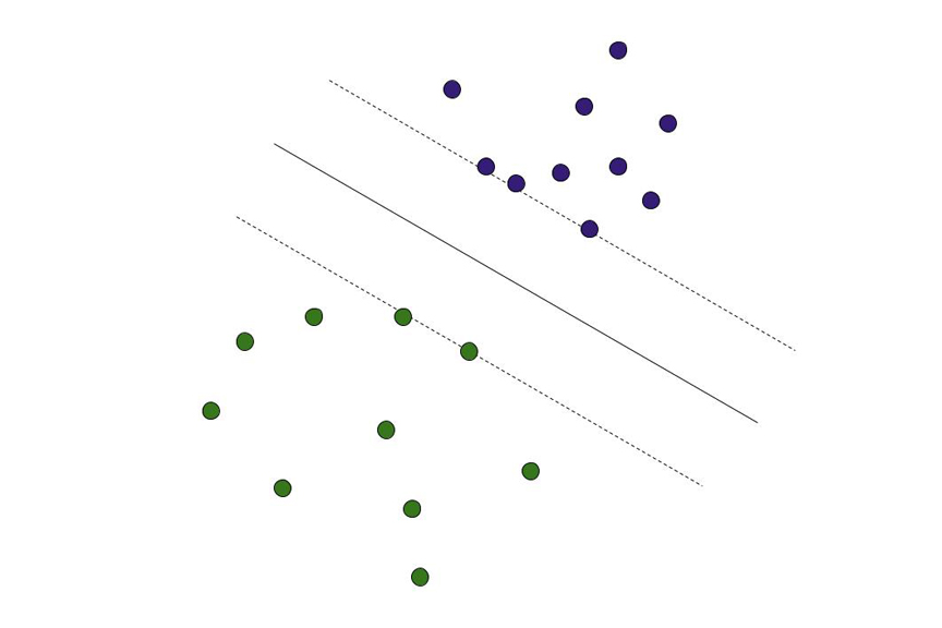
Support Vector Machines (SVMs) are used to turn data sets that are not linearly separable (easily divided into data that indicates a “yes” and data that indicates a “no”) into problems that are linearly separable by transforming the data into higher dimensional spaces and then back. SVMs rely on activation functions to transform the data, and research is still ongoing on optimal choices of activation functions for different problem domains.

Neural Networks

Neural Networks are modeled after how the brain is physically structured. There are neurons and synapses. Neurons receive inputs either from sensory information or from other neurons. Synapses trigger when one of the neurons they are attached to receives input. In Neural Networks, synapses are controlled by the same type of activation functions used by Support Vector Machines. Because the possibilities of connecting neurons is so immense, there are a number of sub-classes of Neural Networks that make them feasible to implement with today’s programming languages and hardware.

• Feed Forward Neural Networks (FNN) have an input layer that is fully connected to a single hidden layer that is then fully connected to an output layer. Neurons within a layer are not connected to each other, and signals only feed “forward’ from the input layer to the output layer.

• Convolutional Neural Networks (CNN) are modified FNNs that are connected in three dimensions. This is really useful for computer vision problems such as object recognition.
• Deep Neural Networks (DNN) are a special class of FNNs that have a very large number of hidden layers. DNNs are important when the problem requires recognizing patterns from very complex inputs but generalized beyond computer vision applications that can use CNNs.

• Recurrent Neural Networks (RNN) have synapses that connect the opposite direction and form cycles. RNNs can be used for processing temporal information since neurons can activate differently depending on how many times they were previously activated.

• Principal Component Analysis (PCA) is the name given to both a training and an inference algorithm. It can only be used in supervised learning but trains very quickly. The algorithm tries to identify which inputs contribute the most information to determine the correct prediction and creates an optimal matrix that when multiplied with the sensory input produces the prediction. Because this reduces the inference capability to problems that can be predicted using linear combinations, it is only applicable in certain problem domains. Here’s a great example.

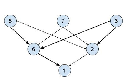
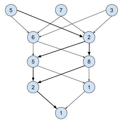
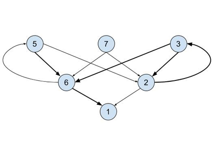
There are many more inference algorithms out there. To decide the correct one for you, you’ll need to deeply understand your problem domain.

Training Algorithms

With the exception of PCA, the above inference algorithms need to optimize its training parameters using an iterative process called fitting. The problem is this: I have some set of inputs and training outputs and I have a function that can transform similar inputs into outputs. Right now it’s coming up with different outputs than the training data. How do I tune my function to give me the right outputs instead? This is a classical mathematical optimization problem. Unfortunately, it’s not easy. We are going to have to head out into the desert with some water strapped on our backs and search for the solution.

Most of the above algorithms can be trained using a variant of Stochastic Gradient Descent (SGD). The algorithm basically works like this:

1. Choose some parameters of the inference algorithm
2. Randomize the training set
3. Compute the output of each input in the training set. Compare the algorithm’s output to the “correct” output in the training data. This is the error margin
4. Adjust the parameters based on the error
5. If the error is small enough, we are done, otherwise go back to step 2

The algorithm is called stochastic gradient descent because we are trying to fall as quickly as possible into the pit of success.

There are a number of potential pitfalls, if you will, with SGD that you need to consider when implementing it. With any optimization problem, there could be small pits (“local minima”) that obscure the large pits (“global minima”). You don’t want your algorithm to stop when it sees the small pit, but continue climbing out of the pit to get to the larger one. With SGD, you can control the learning rate which controls how much the parameter values can change at each iteration of the algorithm.

Validation

Great! We have a trained model that gives us the expected outputs for each example in the training data. Uh oh. Now I have a new input that’s not in any of the previous examples. As luck would have it, my model inferred incorrectly. This is a case of Overfitting. Even though we do want our model to be able to accurately make inferences based on the training data, we don’t want it to be so precise that it loses general predictive power over larger ranges of inputs. There are a number of techniques to avoid over-fitting. The critical component is to split off some of your training data and keep it hidden from the training algorithm. Then give your model a pop quiz using the saved training data and see how it performed. If it accurately predicted the outputs on your validation data set, then it’s less likely that your model overfit the training data. This process is called, you guessed it, Validation!

When you are validating your model, you have to make two decisions. What validation method will you use and what scoring metric will you use? There are only two main types of validation methods so I will cover those here, but there are many scoring metrics such as least mean square error, R, and R squared. Your choice will depend on the types of errors you care or don’t care about in the predictive power of the model but that’s beyond the scope of this article.

Split-Test Validation

Split-Test Validation is the simplest validation method. You split your training data into two parts. The training set is actually provided to the model’s training algorithm. The validation set is used to score the trained model’s predictive power. You will usually want to use the majority of your training examples in the training set. It’s important that the training set has a large variety of samples. If you have a large number of examples (>1000) then you can achieve this simply by shuffling the order of the examples before splitting them. Otherwise you may want to manually pick out representative samples to train with.

Cross-Validation

Cross-Validation (CV) is a good choice when you have a small number of examples because it lets you train with the entire set of examples. The CV algorithm generates multiple partitions of the data and trains a model with each partition and compares it to each other partition. It will then choose the model that scores the best across the validation partitions. Using CV also has an added benefit. Remember those Training Parameters I mentioned previously, way at the beginning of this article? Well, up until now, those had to be chosen by trial and error. With a modification of CV called Grid Search CV or Randomized Search CV, we can optimize those training parameters as well as the inference parameters. Unfortunately, since the CV algorithm doesn’t know anything about the underlying inference algorithm, it can’t use stochastic gradient descent. Instead it performs an exhaustive search of all of the combinations of training parameters and keeps the best trained model. This can be really slow, but is still faster than trying all the permutations by hand.

Ensembles

Any one model has predictive weaknesses based on how the training algorithm works. Why have just one model when you can combine dozens of different models together in an ensemble? Ensembling is how most real world machine learning models are implemented. You can also create your own ensembles manually using any algorithm you choose, even combining models created by hand with trained machine learning models. The possibilities are endless! Sounds easy right? Not. There are some popular ways of auto-ensembling such as:

• Decision Forest: Why have one tree when you can have a whole forest? Forests generate a large number of decision trees based on a permuting the training parameters and then aggregates the results. There are different types of decision forests such as Random Forests and Gradient Boosted Forests depending on the algorithm used to create trees and aggregate their results. Bagging uses a similar algorithm to cross-validation to choose the individual models, and then aggregates the results.
• Voting: The voting method does not automatically generate the ensemble, but is simply an algorithm by which the individual model outputs are aggregated. Each trained model is assigned a weight and then votes on the correct output for the input. The final output is chosen either through weighted average or majority vote. This technique can be used on a heterogeneous set of individual models.

Tools of the Trade

Here are some tools and libraries you can use to create machine learning models without having to learn the underlying math.

• Azure ML by Microsoft: This has some pretty advanced ensemble models and also a very nice visual model designer. It’s a little overkill for making offline predictions, but it’s setup to plugin to a web application really easily. Ideal for large training sets and high volume predictions.
• Amazon ML: The user interface is very difficult to work with and you get very limited control on the feature normalization, training parameters, and inference algorithm compared to Azure ML. But if you are already using AWS infrastructure then this is an option to consider. Ideal for large training sets and high volume predictions.
• Weka: Weka is an open source ML library written in Java. If you are building for Android, desktop, or J2EE scenarios then this is a great choice. It gives you lots of control and is a very deep and broad library.
• scikit-learn: This is a great place to start modeling. The API is extremely robust and it implements some of the more cutting edge algorithms. It’s written in Python so it’s super quick to script in and either build simple low volume web apps, command line applications, or plan for a larger project in one of the other platforms.